Case Study Demo • BioThermR

Introduction

This vignette reproduces the analysis workflow described in the BioThermR manuscript. It demonstrates how to process, visualize, and analyze thermal imaging data from a mouse cold exposure experiment (Normal Diet “ND” vs. Cold Exposed “ND4”).

⚠️ Important Note: Data Availability

The complete dataset used in this case study (30 raw thermal images) is exclusively hosted in the GitHub version of this package due to size constraints. If you installed BioThermR from CRAN, you might miss these files. To fully reproduce the results below, please ensure you have installed the full package from GitHub:

# Install the full version with data from GitHub
if (!require("devtools")) install.packages("devtools")
devtools::install_github("RightSZ/BioThermR")

1. Setup and Installation

First, ensure all dependencies are installed.

# Install dependencies
if (!require("BiocManager", quietly = TRUE))
  install.packages("BiocManager")
BiocManager::install("EBImage")

Load the necessary libraries.

library(ggplot2)
library(ggpubr)
library(BioThermR)

2. Data Loading & Segmentation

# 1. Get the path to the 30 images included with the package
data_folder <- system.file("extdata", package = "BioThermR")

# 2. Read using the batch reading function
obj_list <- read_thermal_batch(data_folder)
length(obj_list)
#> [1] 30

# 3. Use the lapply function to batch call roi_segment_ebimage for segmentation
# Otsu's method is used by default
obj_list <- lapply(obj_list, roi_segment_ebimage)

3. Visualization

Visualize the entire dataset

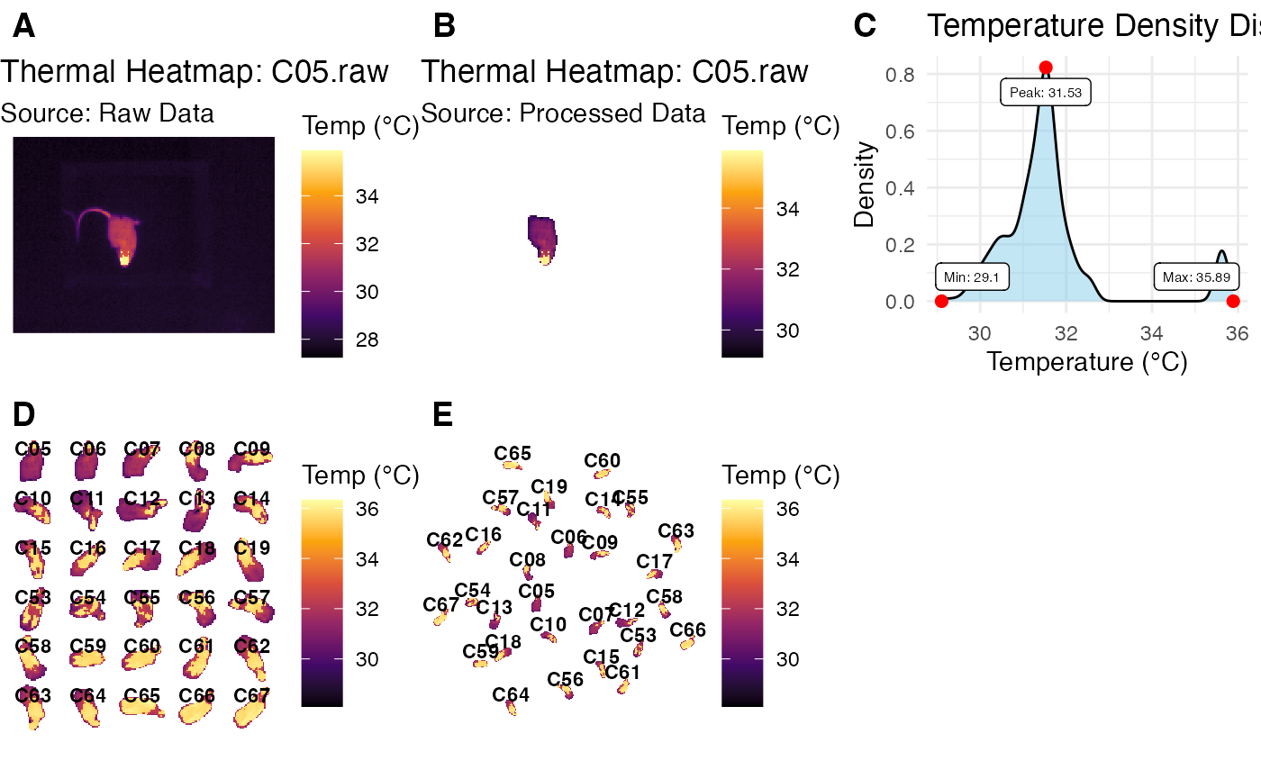
# Display the thermal heatmap of one BioThermR object
p1 <- plot_thermal_heatmap(obj_list[[1]], use_processed = FALSE)
p1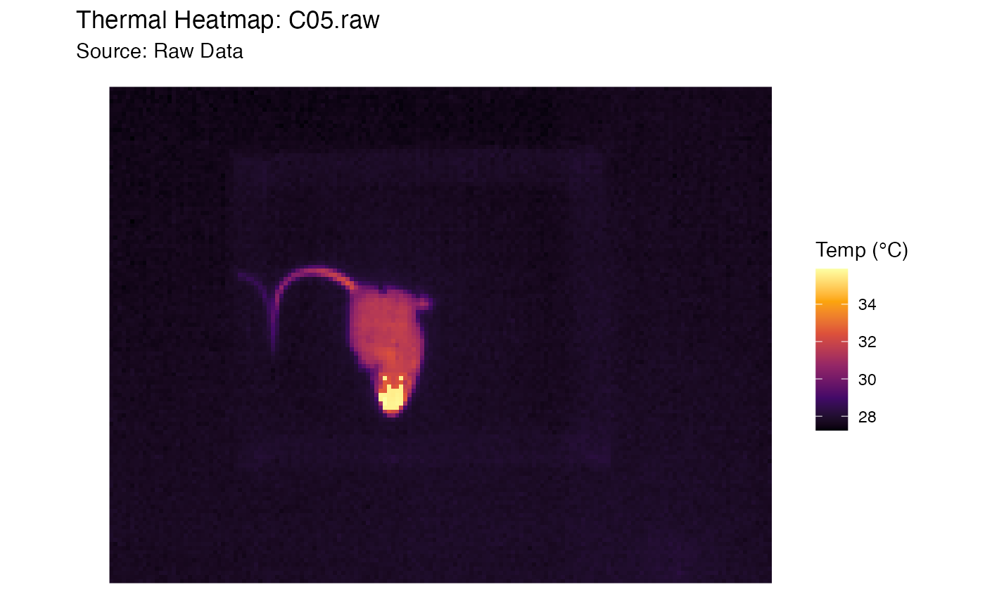

# Display the segmented image of one BioThermR object
p2 <- plot_thermal_heatmap(obj_list[[1]], use_processed = TRUE)
p2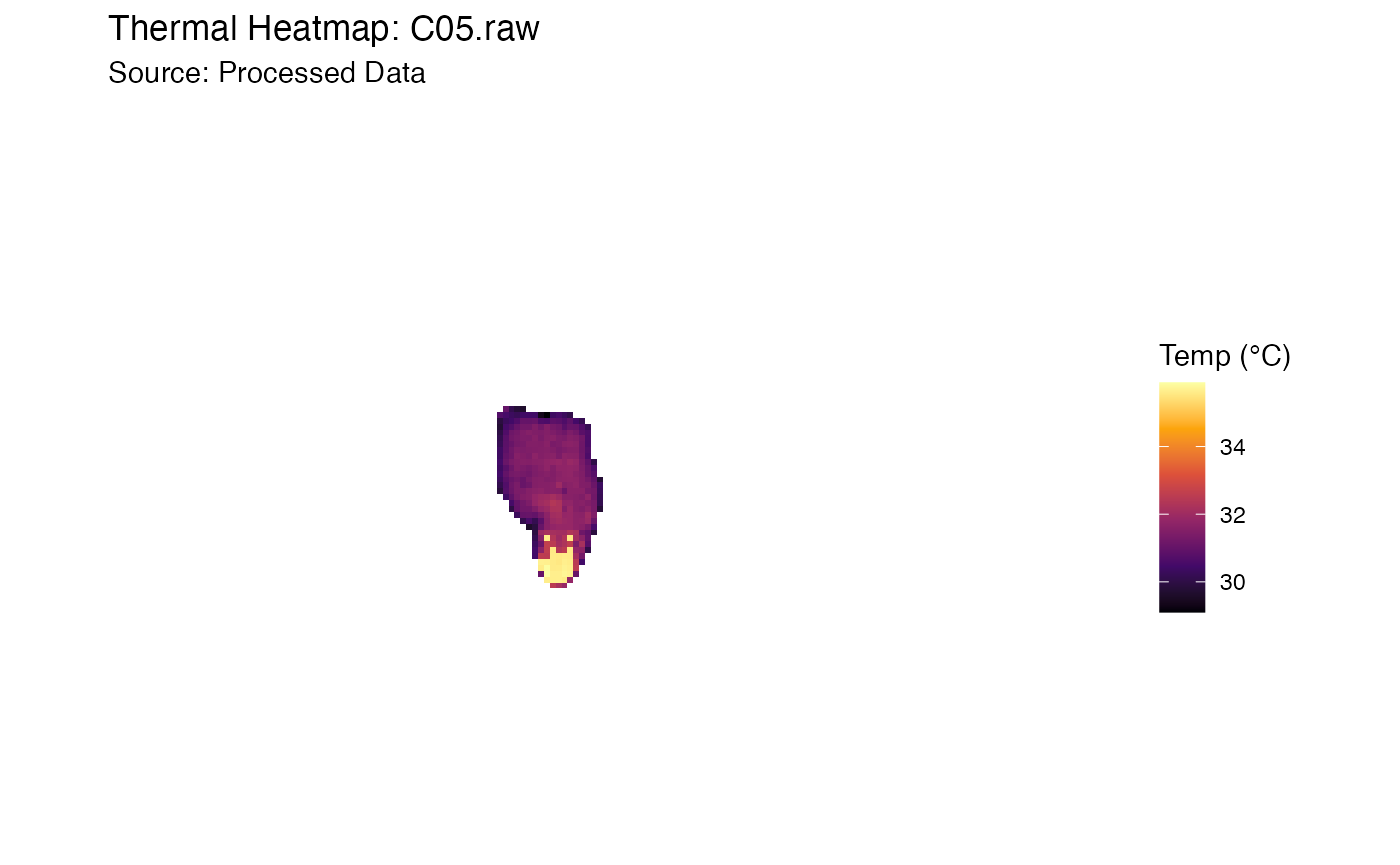

# Display the 3d image of one segmented BioThermR object
plot_thermal_3d(obj_list[[1]])

# Display the ROI density plot of one BioThermR object
p3 <- plot_thermal_density(obj_list[[1]])
p3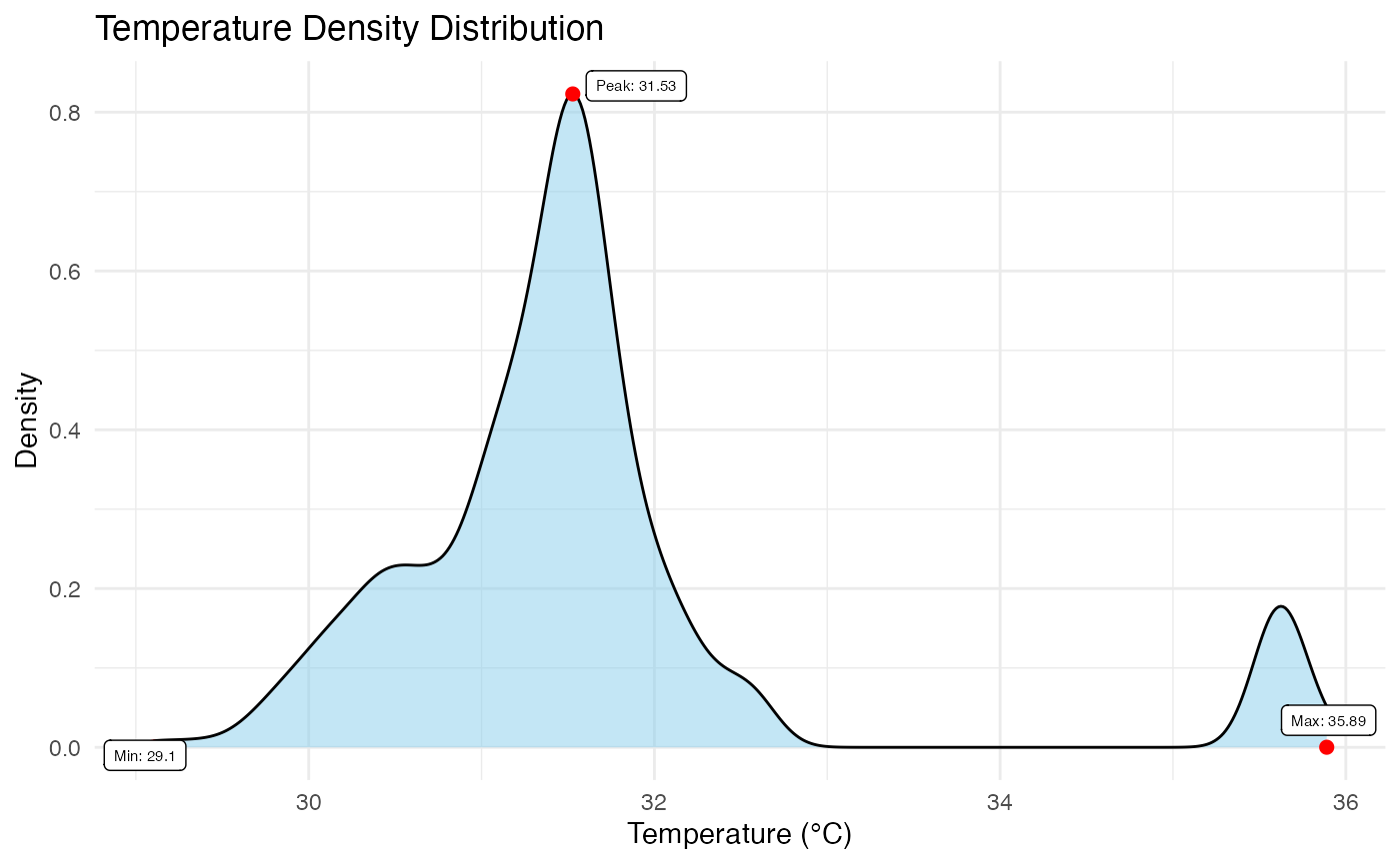

# Display the overall display montage plot
p4 <- plot_thermal_montage(obj_list, ncol = 5, padding = 2, text_size = 3)
p4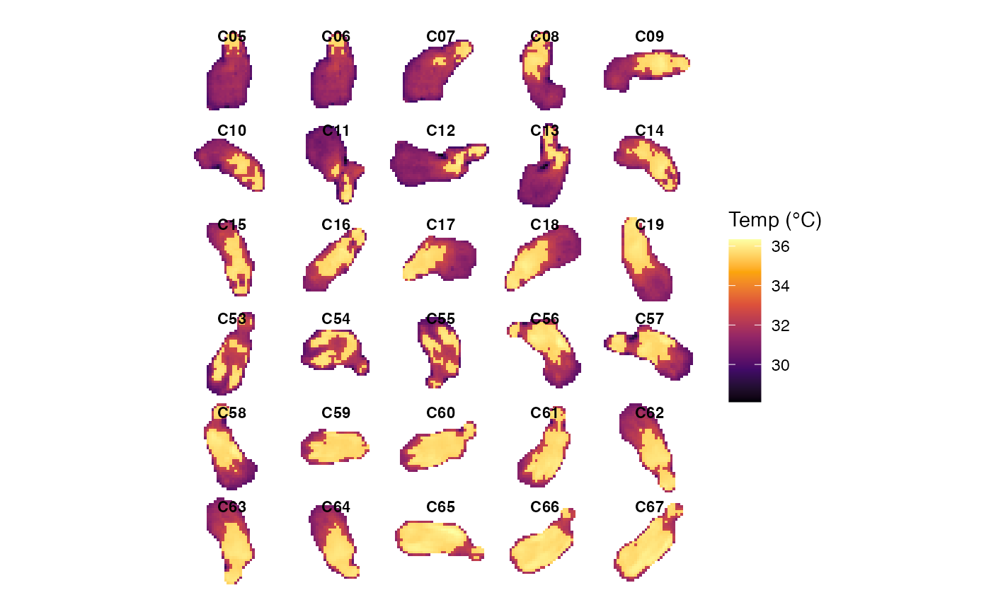

# Display the overall display cloud plot
p5 <- plot_thermal_cloud(obj_list) 
p5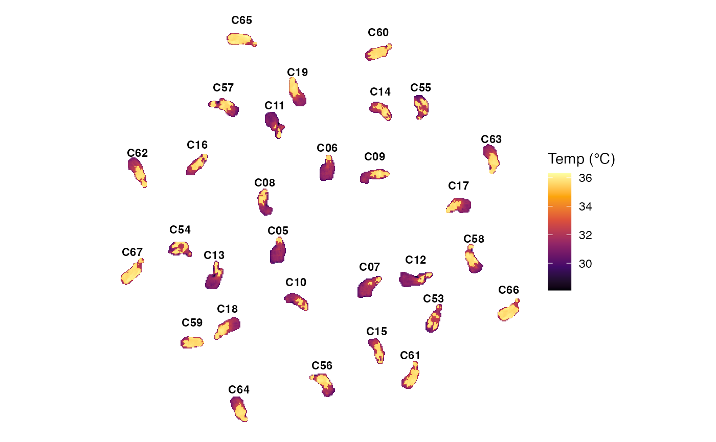

ggpubr::ggarrange(p1,p2,p3,p4,p5,labels = c("A","B","C","D","E"))

4. Statistical Extraction & Compilation

Extract temperature metrics from all images and merge them with clinical grouping data.

# Batch calculate statistics for each BioThermR object
obj_list <- lapply(obj_list, analyze_thermal_stats)

# Compile statistics into a data frame
df <- compile_batch_stats(obj_list)

# Read grouping data and merge
pd_path <- system.file("extdata", "group.csv", package = "BioThermR")
pd <- read.csv(pd_path)
df <- merge_clinical_data(df,pd)

# Aggregate technical replicates (e.g., 3 photos per mouse)
df_new <- aggregate_replicates(df,
                               method = "mean", # use mean method
                               id_col = "Sample", # merge by sample
                               keep_cols = c("Group")
                               )
head(df_new)
#>   Sample Group n_replicates      Min      Max     Mean   Median       SD
#> 1   ND_1    ND            3 29.36788 35.87173 31.70707 31.55465 1.311257
#> 2   ND_2    ND            3 29.19874 35.92883 32.68671 31.84397 1.970498
#> 3   ND_3    ND            3 28.18887 36.03918 31.75590 31.25142 1.650999
#> 4   ND_4    ND            3 30.37368 35.99798 33.32450 32.42096 1.981652
#> 5   ND_5    ND            3 30.59082 35.99695 33.13636 32.18157 1.982310
#> 6  ND4_1   ND4            3 29.27191 35.91896 32.84147 32.21257 1.994384
#>        Q25      Q75       IQR         CV Peak_Density Rep
#> 1 31.07301 31.86817 0.7951624 0.04135084     31.62128   2
#> 2 31.29252 34.58603 3.2935144 0.06027172     31.48556   2
#> 3 30.87554 31.98214 1.1066006 0.05197942     31.09829   2
#> 4 31.73361 35.63418 3.9005693 0.05946340     33.24354   2
#> 5 31.48953 35.62859 4.1390597 0.05982208     31.63697   2
#> 6 31.38211 35.57433 4.1922170 0.06072339     32.02256   2

5. Statistical Comparison

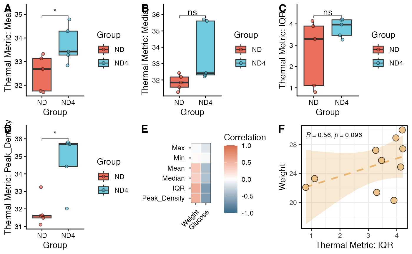
Finally, we compare the thermal metrics between the ND and ND4 groups.

# Display grouping data plots, grouped by Group
my_comparisons <- list( c("ND4", "ND"))
# Mean
s1 <- viz_thermal_boxplot(data = df_new,
                          y_var = "Mean",
                          x_var = "Group") +
  ggpubr::stat_compare_means(comparisons = my_comparisons,
                             method = "t.test",
                             label = "p.signif",
                             hide.ns = FALSE
                             )

# Median
s2 <- viz_thermal_boxplot(data = df_new,
                          y_var = "Median",
                          x_var = "Group")+
  ggpubr::stat_compare_means(comparisons = my_comparisons,
                             method = "t.test",
                             label = "p.signif",
                             hide.ns = FALSE
  )

# IQR
s3 <- viz_thermal_boxplot(data = df_new,
                          y_var = "IQR",
                          x_var = "Group")+
  ggpubr::stat_compare_means(comparisons = my_comparisons,
                             method = "t.test",
                             label = "p.signif",
                             hide.ns = FALSE
  )
# Peak Density
s4 <- viz_thermal_boxplot(data = df_new,
                          y_var = "Peak_Density",
                          x_var = "Group")+
  ggpubr::stat_compare_means(comparisons = my_comparisons,
                             method = "t.test",
                             label = "p.signif",
                             hide.ns = FALSE
  )
ggarrange(s1,s2,s3,s4,ncol = 4,labels = c("A","B","C","D"))