read and plot xpm file

This document demonstrates how to use the xvm package and its functions with sample datasets and plots. It also shows how to read multiple xpm files and arrange their plots using ggpubr.

Note: Ensure dependency packages are installed:

install.packages(c("ggplot2", "stringr", "ggpubr", "ggnewscale"))

Load the xvm package and dependency packages

Load the xvm package:

# Load the xvm package
library(xvm)
#> Error in get(paste0(generic, ".", class), envir = get_method_env()) : 
#>   object 'type_sum.accel' not found

Load other dependency packages:

# Load dependency packages
library(ggplot2)

Read a single xpm file and plot it.

Get Example File Path

Retrieve the path to the example file included in the package:

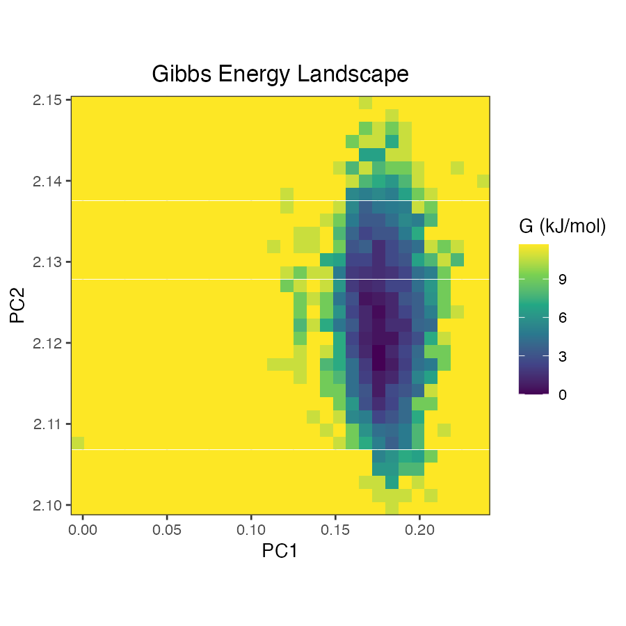
# This example file is an xpm file containing (free energy landscape, FEL) data generated by GROMACS
gibbs_file_path <- system.file("extdata/gibbs.xpm", package = "xvm")

Read the xpm file

# Read the xpm file using read_xpm() function
gibbs_data <- read_xpm(gibbs_file_path)
#> Dimensions parsed: width = 32, height = 32, colors = 50

# The imported xpm file is stored as a list, with the list name corresponding to the file name.
names(gibbs_data)
#> [1] "gibbs.xpm"

The imported xpm file is stored as a list, so you can simply display the data using the str() function.

str(gibbs_data[[1]],max.level = 1)
#> List of 7
#>  $ data        :'data.frame':    1024 obs. of  5 variables:
#>   ..- attr(*, "out.attrs")=List of 2
#>  $ title       : chr "Gibbs Energy Landscape"
#>  $ legend      : chr "G (kJ/mol)"
#>  $ x_label     : chr "PC1"
#>  $ y_label     : chr "PC2"
#>  $ color_map   :List of 50
#>  $ color_values:List of 50

The list contains seven elements, each storing different pieces of information:

$data: a data frame containing the xpm data.

$title: the main title.

$legend: the legend labels.

$x_label: the label for the x-axis.

$y_label: the label for the y-axis.

$color_map: other detailed information about the xpm file, including:

$color_values: other detailed information about the xpm file, including:

Plot the xpm data

# Plot the xpm data using plot_xpm() function
plot_xpm(gibbs_data)

Read multiple xpm Files

The read_xpm() function can accept multiple xpm file paths as a character vector.

# Similarly, you can also read multiple types of xpm files. 
multi_file_path <- dir(system.file("extdata", package = "xvm"))

# Filter out xpm files using stringr package
library(stringr)
multi_file_path <- multi_file_path[str_detect(multi_file_path, ".xpm")]
print(multi_file_path)
#> [1] "entropy.xpm" "gibbs.xpm"

# Set the full xvg file paths
multi_file_path <- file.path(system.file("extdata", package = "xvm"),
                             multi_file_path
                             )

Batch read xpm files

# Read multiple xpm files at once in batch:
multi_data <- read_xpm(multi_file_path)
#> Dimensions parsed: width = 32, height = 32, colors = 50
#> 
#> Dimensions parsed: width = 32, height = 32, colors = 50
names(multi_data)
#> [1] "entropy.xpm" "gibbs.xpm"

Inspect a single xpm file

You can view the information of a single xpm file by indexing the list:

# Check the first xpm file info via indexing
str(multi_data[[1]],max.level = 1)
#> List of 7
#>  $ data        :'data.frame':    1024 obs. of  5 variables:
#>   ..- attr(*, "out.attrs")=List of 2
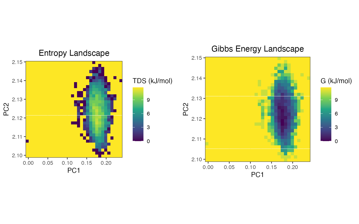
#>  $ title       : chr "Entropy Landscape"
#>  $ legend      : chr "TDS (kJ/mol)"
#>  $ x_label     : chr "PC1"
#>  $ y_label     : chr "PC2"
#>  $ color_map   :List of 50
#>  $ color_values:List of 50

Plot multiple xpm files

Alternatively, use lapply() to generate plots for each xpm file:

# Use lapply() to plot all the xpm files in batch
mutli_xpm_plots <- lapply(multi_data, plot_xpm)

Arrange plots using ggpubr

Finally, arrange all plots into a single layout using the ggarrange() function from the ggpubr package:

# Arrange the plots using ggpubr
library(ggpubr)
ggarrange(plotlist = mutli_xpm_plots)

Plot pseudo-3D from xpm file

For xpm files representing free energy landscapes, xvm also provides a pseudo-3D plotting function plot_xpm_facet().

The upper plot has PC1 on the x axis, G (kJ/mol) on the y axis, and the color indicates the distance in PC2.

The lower plot has PC2 on the x axis, G (kJ/mol) on the y axis, and the color represents the distance in PC1.

# Usage is similar to the plot_xpm() function
plot_xpm_facet(gibbs_data)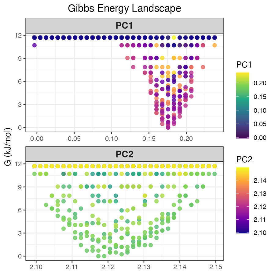

Plot 3D scatter plot from xpm file

xvm also provides a 3D plotting function plot_xpm_3d() using plotly package.

# Usage is similar to the plot_xpm() function
plot_xpm_3d(gibbs_data)